on
Blog 7: Shocks and Unexpected Events
Introduction
This week, I learned about shocks and unexpected events and whether they have an effect on election outcomes. However, my main model for the week did not include shocks and unexpected events and instead focused on incorporating a pooled model. In my model, my dependent variable was Democratic two-party vote share and my independent variables were the average generic ballot score for Democrats, gdp percent difference between Q7 and Q8, incumbency, and the interaction between gdp and incumbency. I was once again able to run the model at the district-level.
What are shocks and unexpected events?
From last week’s lecture, a shock is defined as “a non-systematic event that affects the outcome of an election.” They are often unexpected. An example of a shock in 2022 could be the Dobbs v. Jackson decision where the Supreme Court overruled Roe v. Wade to argue that Constitution of the United States does NOT confer a right to abortion. This could become a shock if, for example, it turns out a lot of angry women and allies out to vote for pro-abortion candidates, than predicted before the Dobbs v. Jackson decision.
Shocks can also be apolitical. For example, Achen and Bartel (2017) examined beach towns in New Jersey and found that beach towns affected by shark attacks voted significantly less for the incumbent than non-beach towns. This finding contributes to an old-held belief that some voters will not vote because of reasons like the weather that day.
Are voters irrational and incompetent?
Thus, this raises the question whether mean voters are irrational and incompetent. In section, I learned that there are cases when voters rationally consider the impact of shocks in their vote. Voters consider what the government could have done better, like better response, relief, and/or preparation. At the same time, there are cases when voters irrationally consider the impact of shocks in their vote. For example, researchers found the effect of partisan bias. When asked which official was to be blamed for September 11, the answer depended on partisanship (Malhotra and Kuo 2008; Healy, Kuo, Malhotra 2014).
When considering shocks systematically, this requires stating a theory and defining the effect: The strength (size) The scope (e.g., where: local vs national, who: engaged vs non-engaged) Persistence
With these three factors in mind, I decided to NOT use shocks in my model. If I was to consider using a shock for 2022 for all 435 districts, I would use the Dobbs v. Jackson decision, but I am concerned about the persistence of its effect as a shock.
Thus, I now turn to the main exploration of this week, which was a pooled model.
Pooled Model
From section slides, I learned that a pool model captures correlation across districts by assuming one set of parameters for all districts to predict each district’s outcome. The benefit of the pooled model is that it relies on less data from each district by “drawing strength” on less data-sparse districts. This was really important to learn as one of the biggest barriers that I have been facing is dealing with less data-sparse districts in my district-level modeling. Thus, I present my pooled model below.
##
## Pooled Linear Regression Model of Democratic Two-Party Vote Share
## ======================================================================
##                                              Dependent variable:
##                                        -------------------------------
##                                        Democratic Two-Party Vote Share
## ----------------------------------------------------------------------
## Generic Ballot for Democrats                      0.515***
##                                                    (0.029)
##
## GDP % Difference from Q6-Q7                       -0.104**
##                                                    (0.052)
##
## Democratic Incumbent in District                  35.945***
##                                                    (0.283)
##
## Interaction between GDP and Incumbency             -0.108
##                                                    (0.070)
##
## Constant                                          10.584***
##                                                    (1.427)
##
## ----------------------------------------------------------------------
## Observations                                       15,498
## R2                                                  0.544
## Adjusted R2                                         0.544
## F Statistic                             4,627.711*** (df = 4; 15493)
## ======================================================================
## Note:                                      *p<0.1; **p<0.05; ***p<0.01
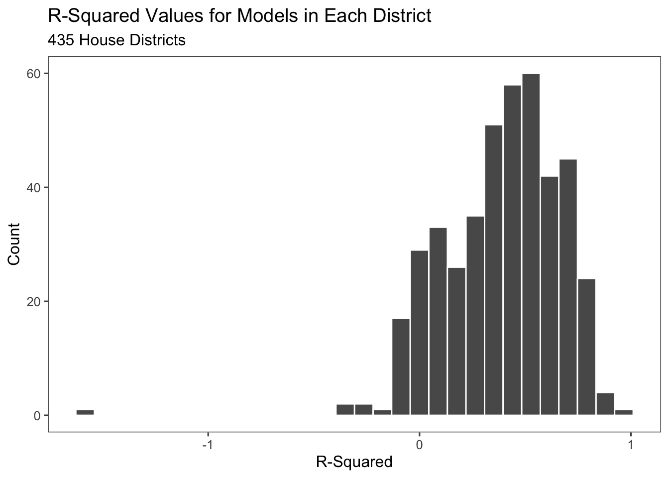
The overall adjusted R squared of this model is 0.544, which is one of the better in-sample evaluations that I have had with a model this semester.

Above, is a distribution of the R squared values by district and compared to last week’s model of voter turnout, this histogram looks more normal and possible. The majority of the R squared values fall between 0 and 1.
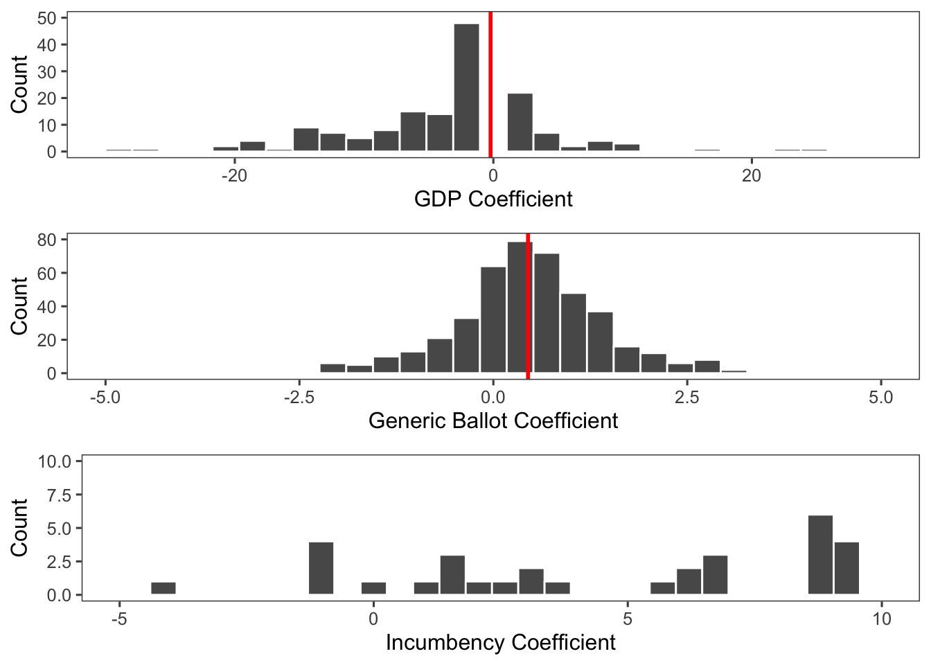
Let’s now take a look at the coefficients. For this week’s pooled model, I decided to explore these variables: 1. Average Generic Ballot Score for Democrats 2. GDP % Difference from Q6-Q7 3. Democratic Incumbency 4. Interaction between Generic ballot and GDP

All variables were statistically significant at p<0.01, except the interaction. As expected, the model shows that as the generic ballot increases by 1 percentage point, Democratic two-party vote share is expected to increase by 0.515 percentage point. In addition, districts with a Democratic incumbent are expected to have a Democratic two-party vote share of 35.945 percentage points more than districts without a Democratic incumbent. However, I am a bit skeptical about how large the difference is. I think this might have occurred because of the way I coded incumbency and the pooled model overfitting for incumbency as a result. This could explain the more sporadic nature of the incumbency coefficient graph. I will address incumbency in my future models in a different way. On the other hand, the model shows that as GDP differences increase by 1 percentage point, the Democratic two-party vote share is expected to decrease by 0.104 percentage point.
Predictions
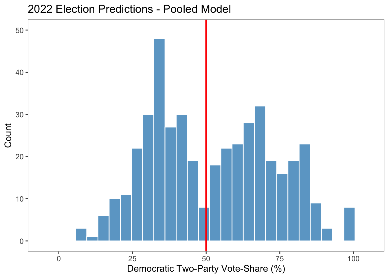
Below is the distribution of the 435 districts’ Democratic two-party vote share based on this pooled model.

This week, I predict that the Republicans will win 212 seats, while the Democrats will win 223 seats, which would result in a Democratic victory in the House. This is definitely an interesting prediction.
My gut feeling does not really necessarily agree with this prediction. Thus, in future models, I plan on readdressing the incumbency variable (perhaps creating multiple incumbency variables at the district-level, House level, and Presidency level) and perhaps adding other variables because my current variables only explain 54.4% of the possible variation. However, I do see a value in using a pooled model because it helps me deal with the data-sparse districts.
Source: Christopher H Achen and Larry M Bartels. Democracy for Realists: Why Elections Do Not Produce Responsive Government, volume 4. Princeton University Press, 2017.